Global Warming Science - www.appinsys.com/GlobalWarming
Atmospheric Circulation
[last update: 2012/10/15]
|
Solar Radiation
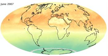
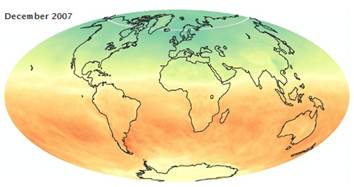
The sun drives the Earth’s atmospheric circulation. Over the course of a year, the hemisphere experiencing summer has a net influx of solar radiation and the hemisphere experiencing winter has a net outflow. The low latitudes around the equator receive influx of solar radiation year-round. This is illustrated in the following figures showing net solar radiation for June and December 2007. [http://earthobservatory.nasa.gov/GlobalMaps/view.php?d1=CERES_NETFLUX_M#]
The above Earth Observatory web site states: “Averaged over the year, there is a net energy surplus at the equator and a net energy deficit at the poles. This equator-versus-pole energy imbalance is the fundamental driver of atmospheric and oceanic circulation.” In general, the heat arrives in the tropics and heads towards the poles (especially the winter pole).
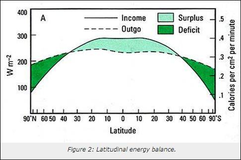
The following figure indicates the net surplus / deficit by latitude. “A large portion of the solar heat at the heat Equator is used for evaporation, changing the water from liquid to gas (water vapor). The heat used isn’t lost but stored as latent heat and transported on the wind systems” [http://drtimball.com/2012/errors-and-omissions-in-major-tropical-climate-mechanism-invalidate-ipcc-computer-models/]
|
|
Atmospheric Circulation
This section examines the general atmospheric circulation pattern of the Earth. The web site: http://www.atmosphere.mpg.de/enid/3sj.html has a good explanation of general atmospheric circulation. The following information and figures in this section are from there.
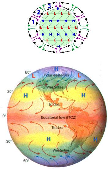
There are three main atmospheric circulation cells as you move from the tropics towards a pole:
1. Tropical cell (Hadley cell) -
Low latitude air moves towards the Equator and heats up. As it heats
it rises vertically and moves polewards in the upper
atmosphere. This forms a convection cell that dominates tropical and
sub-tropical climates. 2. Midlatitude cell (Ferrel cell)
- A mid-latitude mean atmospheric circulation cell for weather named by
Ferrel in the 19th century. In this cell the air flows polewards and towards
the east near the surface and equatorward and in a westerly direction at
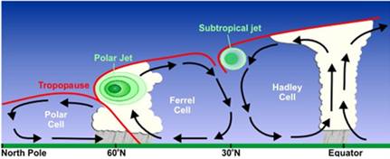
higher levels. 3. Polar cell – At high latitudes air rises, spreads out and travels toward the poles. Once over the poles, the air sinks forming the polar highs. At the surface, the air spreads out from the polar highs. Surface winds in the polar cell are easterly (polar easterlies).
“The tropics receive more heat radiation than they emit, while the polar regions emit more heat radiation than they receive. If no heat was transferred from the tropics to the polar regions, the tropics would get hotter and hotter while the poles would get colder and colder. This latitudinal heat imbalance drives the circulation of the atmosphere and oceans. Around 60% of the heat energy is redistributed around the planet by the atmospheric circulation and around 40% is redistributed by the ocean currents.”
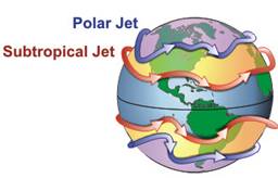
The jet streams are created by these circulation cells. The polar jet stream is generally located in the 50-60 degree N latitude region. The latitudinal position of the jet stream also shifts with the seasons, following the sun – moving towards the pole in the summer. The following figures illustrate the jet stream [http://www.srh.noaa.gov/jetstream//global/jet.htm]
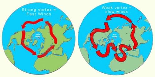
When the polar vortex is strong the jet stream tends to follow a more circular path; when the vortex is weak the jet stream meanders [http://www.john-daly.com/guests/jet.htm]
When the jet stream slows and meanders, it creates blocking patterns (For examples, see: http://www.appinsys.com/GlobalWarming/USsnow_Jan2011.htm and http://www.appinsys.com/GlobalWarming/Russia2010.htm)
|
|
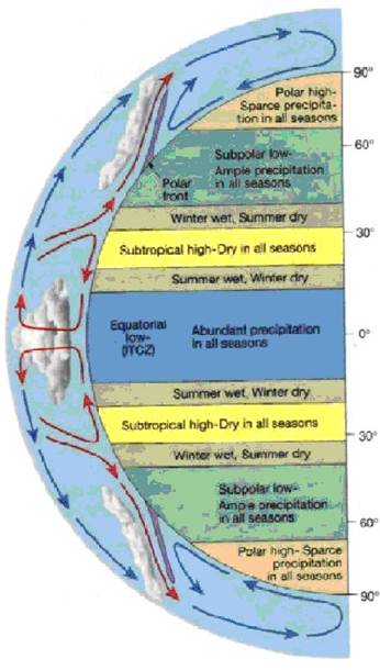
Inter-Tropical Convergence Zone (ITCZ)
The Inter-Tropical Convergence Zone (ITCZ) is formed by the convergence of the trade winds near the equator. It is shown in the first figures above, labeled as the “Equatorial Low (ITCZ)”. “The Inter-Tropical Convergence Zone (ITCZ), appears as a band of clouds, usually thunderstorms, that circle the globe near the equator. The solid band of clouds may extend for many hundreds of miles and is sometimes broken into smaller line segments. The ITCZ follows the sun in that the position varies seasonally. It moves north in the northern summer and south in the northern winter. … In the northern hemisphere the trade winds move in a southwesterly direction, while in the southern hemisphere they move northwesterly. The point at which the trade winds converge forces the air up into the atmosphere, forming the ITCZ.” [http://www.srh.noaa.gov/jetstream//tropics/itcz.htm]
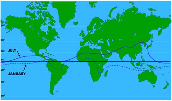
The following figure illustrates the seasonal annual movement of the ITCZ. “The ITCZ moves north during the high-sun season of the Northern Hemisphere, and south during the high-sun season in the Southern Hemisphere. These movements are not perfectly symmetrical above and below the equator, because of the influence of land masses, among other factors.” The seasonal movement of the ITCZ brings the monsoon rains and dry season to tropical areas. [http://www.newmediastudio.org/DataDiscovery/Hurr_ED_Center/Stages_of_Hurricane_Dev/ITCZ/ITCZ.html]
The ITCZ is pulled towards large land masses in the hemisphere where summer is occurring. This implies a gravitational pull by the land masses as well as by the sun.
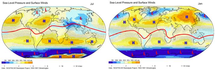
The following figures show a similar (although slightly different) interpretation of the seasonal ITCZ movement also showing sea level pressure (left – July, and right – January [http://www.physicalgeography.net/fundamentals/7p.html]
This web site provides an interesting interactive graphic showing the annual movement of ITCZ: http://daphne.palomar.edu/pdeen/Animations/23_WeatherPat.swf
The seasonal variation of the ITCZ and the Hadley circulation is abrupt: “the seasonal migration of the global zonal-mean intertropical convergence zone (ITCZ) is not smooth, but jumps from the winter hemisphere to the summer hemisphere. The abrupt migration is within 10 days. Detailed analyses reveal that the phenomenon of the abrupt seasonal migration of the ITCZ mainly exists over particular tropical domains, such as Indian Ocean, western and central Pacific, and South America, which gives the rise of the jump of the global zonal-mean ITCZ. Because the ITCZ constitutes the ascending branch of the Hadley circulation, we also examine whether there exists such an abrupt seasonal change in the Hadley circulation. It is found that the intensity of the Hadley cells evolves smoothly with time. However, the horizontal scales of the Hadley cells demonstrate abrupt seasonal changes, corresponding to the abrupt seasonal migration of the global ITCZ. The winter cell extends rapidly across the equator, while the summer cell rapidly narrows. This suggests that the solsticial cell is the dominant component of the Hadley circulation, and that the equinoctial symmetric pattern is ephemeral.” [http://www.agu.org/pubs/crossref/2007/2007GL030950.shtml]
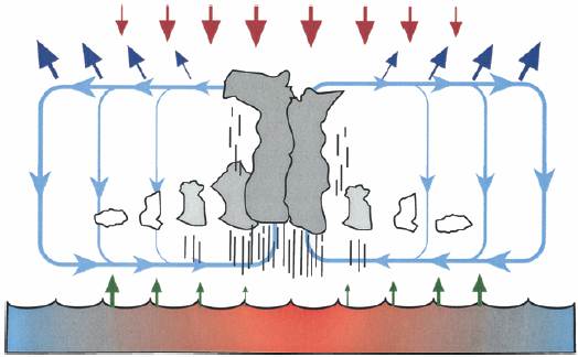
The ITCZ follows the sun. The following figure shows “the ITCZ in the context of the water and energy cycles of the tropics. The downward arrows at the top of the atmosphere depict the incoming solar energy from the Sun. The upward arrows leaving the surface of the ocean depict the transfer of heat and moisture from the ocean to the near-surface air via sensible heat and latent (i.e., evaporative) heat fluxes. The upward arrows at the top of the atmosphere denote this energy being transferred back to space via radiative heat loss.” [http://hydro.jpl.nasa.gov/other/itcz.ency.galley.pdf]
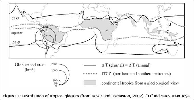
The ITCZ also helps define the area of tropical glaciers. Tropical glaciers “lie within regions where three zones coincide (Figure 1): (1) the astronomic tropics (between the Tropics of Cancer and Capricorn), (2) the oscillation zone of the Intertropical Convergence Zone (ITCZ), and (3) a zone where the diurnal amplitude of air temperature exceeds the annual amplitude” [http://www.phys.uu.nl/~pelt0108/karthaus09/lecturenotes/ThomasMoelg.pdf] The following figure is from the same source.
“The annual cycle of tropical climate is due to the annual cycle of moisture only: humidity, clouds, and precipitation (cf. fundamentals of tropical climate and meteorology as presented by Hastenrath (1991) and Asnani (1993)). In general, this cycle results from the north-south oscillation of the ITCZ, one of the main circulation patterns in our climate system. The ITCZ is a zone of strong convection and rainfall that passes equatorial regions twice a year, and reaches the boundary regions of its oscillation (outer tropics) only once a year.”
|
|
ITCZ Seasonal Continental Movement in Africa
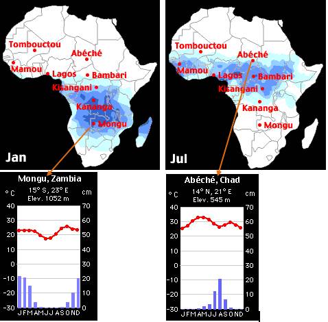
The seasonal movement of the ITCZ is illustrated for Africa – January (left) and July (right) (from [http://people.cas.sc.edu/carbone/modules/mods4car/africa-itcz/index.html]) The movement of the ITCZ causes rainy seasons at opposite times of the year for the northern and southern reaches. The northern edge of the northern-summer ITCZ is the Sahel area of Africa – i.e. the northern edge of the ITCZ controls the southern extent of the Sahara desert.
|
|
ITCZ Seasonal Pacific Movement and Relation to El Nino
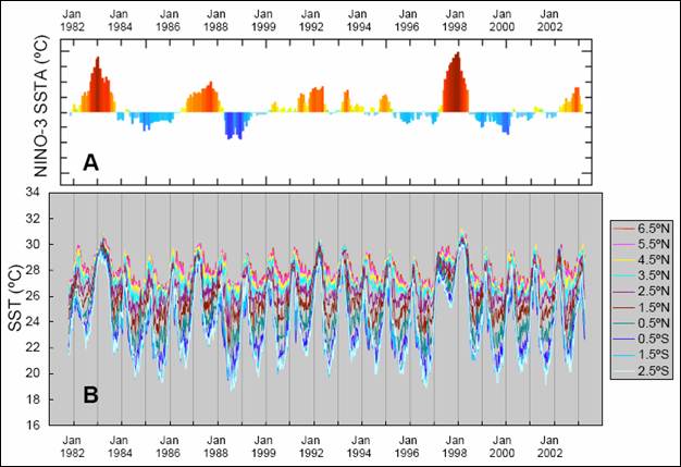
The seasonal movement of the ITCZ in the Eastern Pacific is illustrated with sea surface temperature (SST) gradients. “Through observations made during the instrumental era, it is now understood that at least over interannual time scales associated with the El Niño/Southern Oscillation (ENSO), the position of the Pacific ITCZ varies predictably with the phase of ENSO (e.g., Deser and Wallace 1990). El Niño events are typically marked by equatorward expansion of the ITCZ, whereas La Niña occurrences are marked by a more northerly ITCZ.” This is illustrated in the following figure, comparing Nino 3 SST anomalies (top) with the weekly SST gradient from 7N to 3S at 90W: “A weak gradient in the early part of the year occurs under the influence of the “doldrums” while the ITCZ [Inter-Tropical Convergence Zone] is positioned near the equator. Later in the year, as the ITCZ shifts north, the southeast trades across the equator strengthen and drive enhanced upwelling, hence a strong gradient develops. Prominent El Niño anomalies (e.g., 1982–83, 1987, 1997–98) are marked by unusually weak gradients and more southerly ITCZ, whereas La Niñas (e.g., 1988) are marked by an enhanced and longer-persisting SST gradient, and more northerly ITCZ.” [http://shadow.eas.gatech.edu/~jean/Koutavas2004.pdf]
|
|
ITCZ Century-Scale Movement
The ITCZ not only moves north and south with the annual seasonal change in the main location of solar influx, it has also moved south and north over multi-century time-scales.
“Southward Movement of the Pacific Intertropical Convergence Zone AD1400-1850”, Sachs et al, Nature Geoscience 2009 [http://www.nature.com/ngeo/journal/v2/n7/full/ngeo554.html]: “evidence from continental Asia, Africa and the Americas suggests that it has shifted substantially during the past millennium, reaching its southernmost position some time during the Little Ice Age (AD 1400–1850). … the Pacific intertropical convergence zone was south of its modern position for most of the past millennium, by as much as 500 km during the Little Ice Age. A colder Northern Hemisphere at that time, possibly resulting from lower solar irradiance, may have driven the intertropical convergence zone south.” [http://www.atmos.washington.edu/~david/Sachs_etal_2009.pdf]
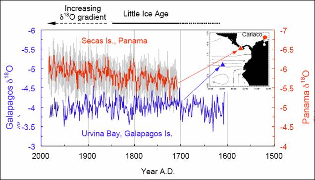
Further evidence of the northward ITCZ shift since the Little Ice Age (LIA) is provided in the following figure (from [http://shadow.eas.gatech.edu/~jean/Koutavas2004.pdf]) which states: “Evidence from Cariaco indicates a northward shift of the ITCZ since the end of the LIA (Haug et al. 2001), which is reflected in the Pacific by the increasing isotopic gradient between the two corals since the mid-nineteenth century.” The diverging trend between the Galapagos and Secas Island indicate that the ITCZ has been moving northward.
Haug et al (“Southward Migration of the Intertropical Convergence Zone Through the Holocene”, Science Vol.293, 2001 [http://www.whoi.edu/science/GG/paleoseminar/pdf/haug01.pdf]): “The Cariaco record, when combined with other records from South America, unambiguously shows that climate changes in Central and South America over the course of the Holocene are due at least in part to a general southward shift of the ITCZ.”
Poore et al (“Century-scale movement of the Atlantic Intertropical Convergence Zone linked to solar variability”, Geophysical Research Letters, Vol 31, 2004) [http://www.cfa.harvard.edu/~wsoon/SunClimate09-d/PooreQuinnetal04GRL.pdf]: “The abundance of the planktic foraminifer Globigerinoides sacculifer in Gulf of Mexico (GOM) sediments is a proxy for the influx of Caribbean surface waters (the Loop Current) into the GOM. Penetration of the Loop Current into the GOM is related to the position of the Intertropical Convergence Zone (ITCZ): northward migration of the ITCZ results in increased incursion of the Loop Current into the GOM; …the average position of the ITCZ and thus Holocene century-scale variability in the Caribbean-GOM region is linked to solar variability.”
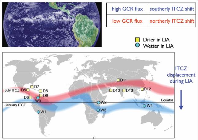
CERN’s Jasper Kirby has suggested that the movement of the ITCZ is related to changes in galactic cosmic ray flux [http://indico.cern.ch/getFile.py/access?resId=0&materialId=slides&confId=52576] (following figure from his referenced presentation).
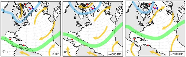
The following figure shows the July ITCZ long term migration and is from Figure 3 in Knudsen et al (“Tracking the Atlantic Multidecadal Oscillation through the last 8,000 years”, Nature Communications, 2011, [http://www.nature.com/ncomms/journal/v2/n2/full/ncomms1186.html])
|
|
Sixty-Year Cycle
I was reading Ronald Wright’s travel book “Time among the Maya”, published in 1989. Wright arrived in Flores on the island in Lake Peten Itza and the proprietor told him about the fluctuating lake level: “Look at those poor fools! People come here and they don’t listen to the older folk. We Peteneros – we know the lake has a cycle every fifty years or so.”
Hillesheim et al (“Climate change in lowland Central America during the late deglacial and early Holocene”, Journal of Quaternary Science, 2005 [http://snre.ufl.edu/graduate/files/publicationsbyalumni/Hillesheim,%20Buck%20et%20al%202005.pdf]): “the observed changes in lowland Neotropical precipitation were related to the intensity of the annual cycle and associated displacements in the mean latitudinal position of the Intertropical Convergence Zone … Lake Pete´n Itza´ is a terminal basin fed by precipitation, subsurface groundwater inflow, and a small input stream in the southeast. The basin is effectively closed, lacking any surface outlets, although some downward leakage may occur. Lake Pete´n Itza´ is situated in a climatically sensitive region where the amount of rainfall is related to the seasonal migration of the Intertropical Convergence Zone (ITCZ) and Azores–Bermuda high-pressure System. Lake Pete´n Itza´’s volume is sensitive to precipitation changes and has fluctuated markedly in the recent past. For example, mean annual rainfall during the period from 1934 to 1942 was relatively high (2055mm/yr) and resulted in increased lake levels and flooding (Deevey et al., 1980). In contrast, the early to mid-1970s were relatively dry (mean annual rainfall 1415mm/yr) resulting in lower lake levels. During the late 1970s lake level rose again in response to increased precipitation continuing until the early 1990s at which time the trend reversed.” This is an approximately 60-year cycle.
Knudsen et al (“Tracking the Atlantic Multidecadal Oscillation through the last 8,000 years”, Nature Communications, 2011, [http://www.nature.com/ncomms/journal/v2/n2/full/ncomms1186.html]): “Our analyses further suggest that the coupling from the AMO to regional climate conditions was modulated by orbitally induced shifts in large-scale ocean-atmosphere circulation. … these sites [in central America] seem to have become more sensitive to changes in ITCZ, and hence the AMO, as even slight changes in North Atlantic SST can cause N-S shifts in the ITCZ and thus in rainfall.”
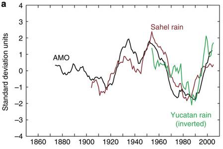
The following figure is from Figure 2 in Knudsen et al. The Yucatan site is Lake Chichancanab
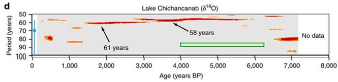
The following figure is from Figure 5 in Knudsen et al showing the spectrogram highlighting the 58-61 year periodicity in the Lake Chichancanab data.
|
|
Atmospheric Angular Momentum / Length of Day
The atmospheric angular momentum (AAM) and the length of day (LOD) are interconnected. (see: [http://www.livescience.com/178-spin-earth-rotation.html])
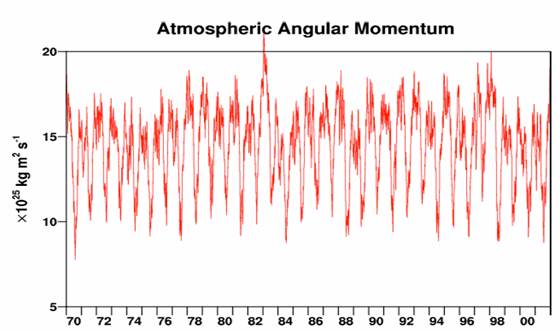
“The angular momentum of the atmosphere is a signal that changes on many climate time scales due to the motion of winds and to atmospheric mass redistribution; angular momentum is exchanged, moreover, across the atmosphere’s lower boundary. The atmospheric angular momentum signal responds to certain signals like the El Niño, which is observed in some geodetic properties such as Earth’s rotation rate, reckoned by the small changes in the length of day, and also in the motions of the pole.” [http://ams.confex.com/ams/pdfpapers/55763.pdf]
The following figures are from the above source (figures 4 – top – and 7 – bottom) “The maxima in Fig. 4 occur during occurrences of El Niño when anomalous westerly zonal flow throughout much of the tropics and subtropics occurs, sometimes extending as well into higher latitudes; the events in 1983 and 1997-98 are contain record high values of the angular momentum index. The global maxima derive from momentum anomalies that often start in the lowest latitudes and propagate toward poleward”
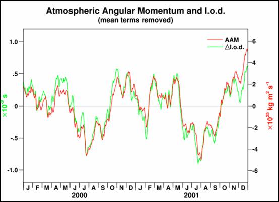
“The global axial angular momentum is very strongly connected to values in the length of day; such connections occur on time scales between days and several years (Fig. 7).”
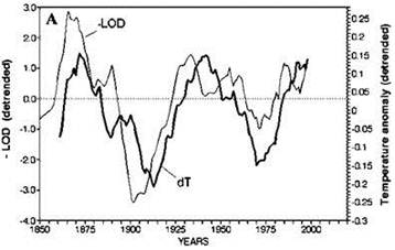
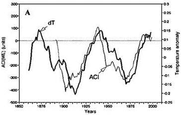
A UN Food and Agricultural Organization (FAO) report on “Climate Change and Long-Term Fluctuation of Commercial Catches”, 2001 [ftp://ftp.fao.org/docrep/fao/005/y2787e/y2787e01.pdf] provides the following figures comparing detrended length of day (LOD) and Atmospheric Circulation Index (ACI) with detrended global temperature anomaly (from same FAO study).
The FAO report states the LOD is “a geophysical index that characterizes variation in the earth rotational velocity … Spectral density analysis of the LOD time series for 1850-1998 revealed clear, regular fluctuations with an approximate 60-year period length”
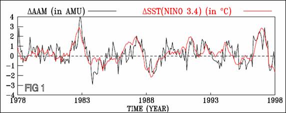
The following figure compares the change in atmospheric angular momentum (AAM) with the change in Nino 3.4 sea surface temperatures [http://www-pcmdi.llnl.gov/projects/cmip/cmip_subprojects/Huang/huang_proposal.pdf] The atmospheric angular momentum (AAM) results from the Earth’s atmosphere and the planet itself rotating at different speeds and causes fluctuation in the length of a day, as well as affecting the polar wobble.
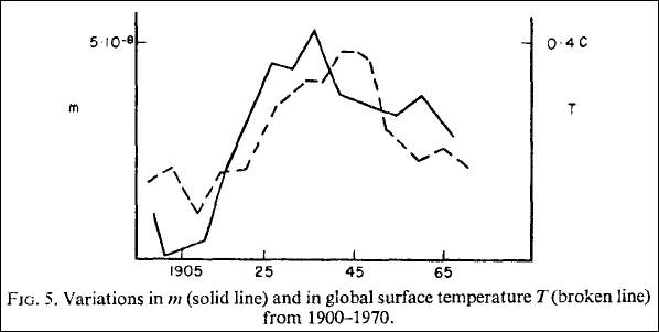
Lambeck and Cazanave “Long Term Variations in the Length of Day and Climatic Change” Geophysics Journal, 1976 [http://people.rses.anu.edu.au/lambeck_k/pdf/37.pdf] stated: “The long-period (greater than about 10 yr) variations in the length-of-day (LOD) observed since 1820 show a marked similarity with variations observed in various climatic indices; periods of acceleration of the Earth corresponding to years of increasing intensity of the zonal circulation and to global-surface warming: periods of deceleration corresponding to years of decreasing zonal-circulation intensity and to a global decrease in surface temperatures.”
The following figure is from that paper (m = change in LOD / LOD).
“the continuing deceleration of m for the last 10 yr suggests that the present period of decreasing average global temperature will continue for at least another 5-10 yr. Perhaps a slight comfort in this gloomy trend is that in 1972 the LOD showed a sharp positive acceleration that has persisted until the present, although it is impossible to say if this trend will continue as it did at the turn of the century or whether it is only a small perturbation in the more general decelerating trend.” So in 1976, before the CO2 craze, they recognized the connection between AAM/LOD and temperature.
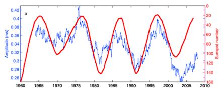
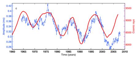
The following figures compare the length of day amplitude (blue) with sunspot number (top) and cosmic rays (bottom) [http://www.nipccreport.org/articles/2010/aug/19aug2010a7.html] (See also http://www.agu.org/journals/ABS/2010/2010GL043185.shtml)
|
|
Tropical SST Drives Global Atmospheric Circulation
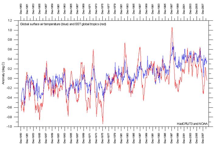
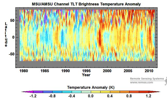
The following figure compares tropical sea surface temperature (SST) in the tropics (red - 10N-10S x 0-360) with global average surface air temperature (blue). (from [http://www.climate4you.com/SeaTemperatures.htm])
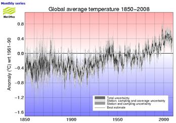
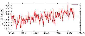
The following figures show global average temperature anomalies (left, from [http://hadobs.metoffice.com/hadcrut3/diagnostics/global/nh+sh/]) and sea surface temperature anomalies for the tropical pacific area of 20N – 20S x 90W – 120E (right, from the ERSST v3b SST data plotted at [http://climexp.knmi.nl/]).
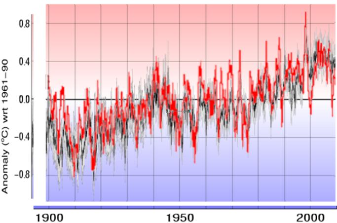
The following figure combines the above two. It is evident from this figure that the tropical Pacific Ocean sea surface temperature drives the global air temperature.
See: http://www.appinsys.com/GlobalWarming/TropicalSST.htm
http://www.ssmi.com/msu/msu_data_description.html
A paper written 40 years ago provides some insight that seems to have been lost in modern climate studies. “Polar Ice and the Global Climate Machine” Joseph Fletcher , 1970 [http://books.google.com/books?id=EAcAAAAAMBAJ&pg=PA40&lpg=PA40#v=onepage&q&f=false]
|
|
Magnetic Connection
The following information is from a 2006 NASA article “First Global Connection Between Earth and Space Weather Found” [http://www.nasa.gov/centers/goddard/news/topstory/2006/space_weather_link.html]
“The ionosphere is formed by solar X-rays and ultraviolet light, which break apart atoms and molecules in the upper atmosphere, creating a layer of electrically-charged gas known as plasma. The densest part of the ionosphere forms two bands of plasma close to the equator at a height of almost 250 miles.”
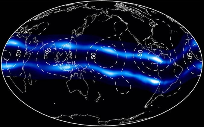
“the team discovered four pairs of bright regions where the ionosphere was almost twice as dense as the average. Three of the bright pairs were located over tropical rainforests with lots of thunderstorm activity -- the Amazon Basin in South America, the Congo Basin in Africa, and Indonesia. A fourth pair appeared over the Pacific Ocean. … The single pair of bright zones over the Pacific Ocean that is not associated with strong thunderstorm activity shows the disruption is propagating around the Earth, making this the first global effect on space weather from surface weather that's been identified.”
The following figure is “a false-color image of ultraviolet light from two plasma bands in the ionosphere that encircle the Earth over the equator. Bright, blue-white areas are where the plasma is densest. Solid white lines outline the continents; Africa is on the left, and North and South America are on the right. Dotted white lines mark regions where rising tides of hot air indirectly create the bright, dense zones in the bands.”
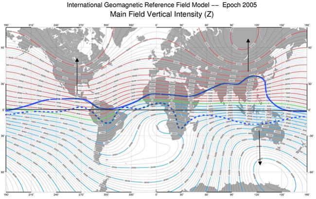
The plasma bands above do not follow the Earth’s equator, but rather, follow the magnetic equator and are approximately +/-10 degrees north and south of the magnetic equator. The following figure shows the Earth’s magnetic field (vertical intensity), showing the magnetic equator (green line) as well as the ITCZ seasonal variation (blue lines). [ftp://ftp.ngdc.noaa.gov/Solid_Earth/Mainfld_Mag/images/Z_map_mf_2005_large.jpeg]
|
|
|