Global Warming Science - www.appinsys.com/GlobalWarming
[last update: 2011/02/15]
|
The ozone hole is a stratospheric phenomenon that varies throughout the year, as well as spatially on the Earth. In the mid-latitudes (35°-60°), the ozone depletion is in the range of 3 – 5 %: “Outside polar regions, ozone depletion has been relatively small, hence, in many places, increases in UV due to this depletion are difficult to separate from the increases caused by other factors, such as changes in cloud and aerosol.” [Ref.1 – United Nations / World Meteorological Organization Scientific Assessment Report on Ozone 2006 - cited at the end of this document]. The major ozone depletion occurs seasonally over the poles, with the Antarctic ozone depletion being larger. The polar holes are seasonal phenomena – they occur in the respective polar winter when the sun does not reach the pole and they reach the maximum size at the end of the winter. The arrival of the sun with the onset of spring reduces the ozone hole and eliminates it during the summer.
According to the Australian Bureau of Meteorology, “The initial monitoring of ozone was driven by curiosity about the circulation in the upper levels of the atmosphere. Because measurements of total ozone were observed to be related to the passage of weather systems, it was used for many years as an aid to weather forecasting. Now, of course, the focus is very much on the depletion of the ozone layer due to anthropogenic pollutants and the ensuing negative biological impacts.” [http://www.bom.gov.au/inside/oeb/atmoswatch/aboutozone.shtml]
This document contains the following sections:
|
|
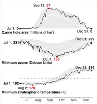
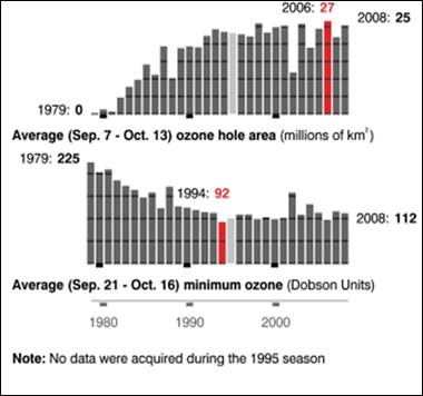
The following figures show historical data on the Antarctic ozone hole since satellite observations began in 1979 [http://ozonewatch.gsfc.nasa.gov/]. The left figure shows the size of the ozone hole (top), minimum ozone (center) and minimum stratospheric temperature (bottom) with the black line showing the 2008 data and the gray area showing the range since 1979. The right figure shows the trend in the size of the ozone hole (top) and the minimum ozone (lower). The hole expanded from 1979 to 1990 and has leveled off for the last almost 20 years.
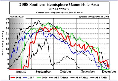
The following figure shows the seasonal occurrence of the Antarctic ozone hole for 2006, 2007 and 2008 along with the 1998-2007 mean and minimum and maximum extents. The annual maximum depletion is in mid-September. [http://www.cpc.noaa.gov/products/stratosphere/polar/gif_files/ozone_hole_plot.png].
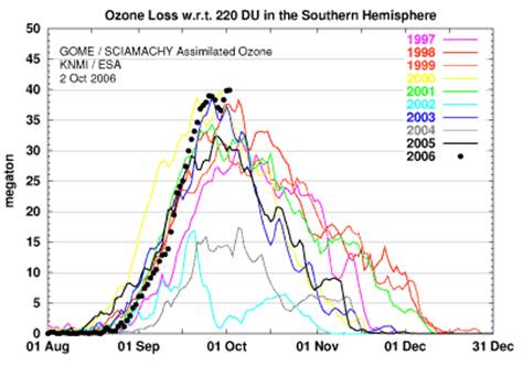
The following figure shows the same as above but incorporating more years and in terms of megatons rather than area [http://www.physorg.com/news79016486.html].
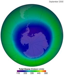
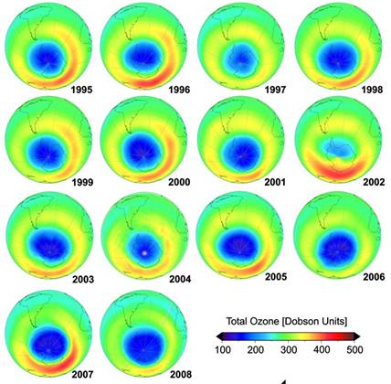
The following figure shows the ozone hole in September 2008 (left) [http://ozonewatch.gsfc.nasa.gov/monthly/monthly_2008-09.html] and (right) from 1995 to 2008 [http://www.theozonehole.com/ozoneholehistory.htm]
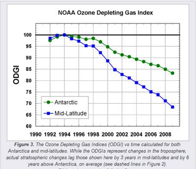
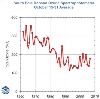
The following figures show (left) the Ozone Depleting Gas Index (ODGI) for the Antarctic and the mid-latitudes [http://www.esrl.noaa.gov/gmd/odgi/] and (right) the Antarctic total ozone in October [http://www.esrl.noaa.gov/gmd/dv/spo_oz/ozdob.html] (The ODGI is defined as 100 at the peak in EECl, and zero at the EECl level corresponding to when recovery might be expected in the mid-latitude stratosphere.) The ODGI has declined since the Montreal Protocol was implemented in 1987 (left), and the ozone level has leveled off at the 1990 level. This is also indicated by the first figure in this document which shows the size of the Antarctic ozone hole remains relatively unchanged since 1990.
A 2009 article “Increasing Antarctic Sea Ice Extent Linked to Ozone Hole” [http://www.sciencedaily.com/releases/2009/04/090421101629.htm] states: “Antarctic sea ice has increased by a small amount as a result of the ozone hole delaying the impact of greenhouse gas increases on the climate of the continent.” Logic escapes them as they search for more reasons why the climate models fail in their CO2-based predictions for Antarctica. The following figure shows the mid-April 2008 to mid-April 2009 Antarctic sea ice anomalies showing the typical seasonal pattern over the last decade. [http://arctic.atmos.uiuc.edu/cryosphere/IMAGES/current.365.south.jpg]. Contrary to the article, the increased ice anomalies have been occurring in the opposite phase from the ozone depletion – the minimum in the ice cycle occurs in September, corresponding to the maximum in ozone depletion.
Further information on the south polar “ozone hole” can be found at: [http://www.cpc.ncep.noaa.gov/products/stratosphere/polar/polar.shtml]
|
|
The WMO ozone report [Ref.1] makes the following statements about the Arctic ozone hole:
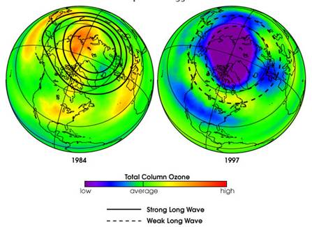
The following figure compares Arctic ozone in February 1984 and 1997 [http://earthobservatory.nasa.gov/IOTD/view.php?id=1771] “long waves move up from the lower atmosphere (troposphere) into the stratosphere, where they dissipate. When these waves break up in the upper atmosphere they produce a warming of the polar region. So, when more waves are present to break apart, the stratosphere becomes warmer. When fewer waves rise up and dissipate, the stratosphere cools, and more ozone loss occurs.”
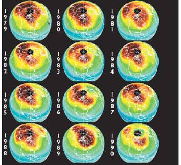
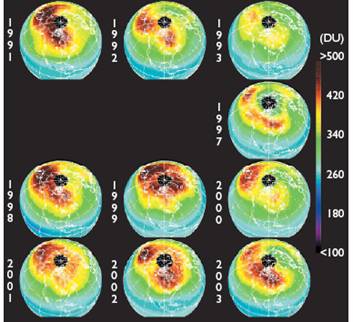
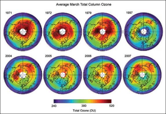
The following figure compares Arctic ozone for March from 1979 – 2003 [http://www.acia.uaf.edu:16080/PDFs/ACIA_Science_Chapters_Final/ACIA_Ch05_Final.pdf]
Updated March total column ozone [http://downloads.climatescience.gov/sap/sap2-4/sap2-4-final-ch3.pdf]:
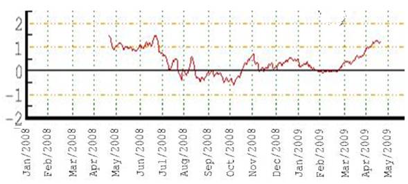
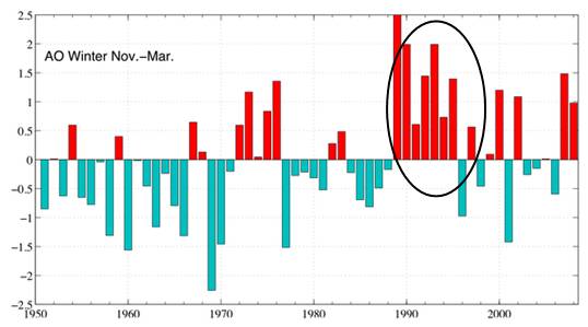
The following figure shows the winter Arctic Oscillation (AO) for 1950 - 2008 [http://www.arctic.noaa.gov/detect/climate-ao.shtml]. The positive AO seems to correspond to lower ozone, lagged by one year. The AO started a strong positive phase in 1989 and the ozone decreased starting in 1990 as shown above.
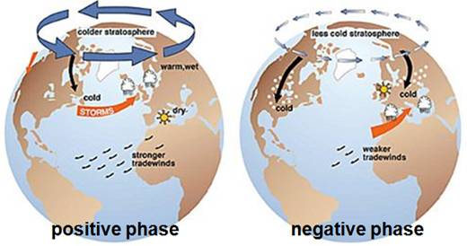
The following figures show the effect of positive AO (left) and negative AO (right) [http://biogeo.botanik.uni-greifswald.de/fileadmin/user_upload/_temp_/Martin/lesson/CC_Wilmking_05.ppt]. The colder stratosphere associated with the positive AO results in reduced ozone.
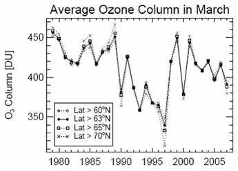
The following figure shows the Arctic ozone in March for 1979 – 2007 (left) [http://hal.archives-ouvertes.fr/docs/00/29/64/14/PDF/acp-8-251-2008.pdf] and (right) comparing that to the multivariate El Nino / Southern Oscillation Index (MEI) with ozone lagged by one year (i.e. ENSO leads by one year). The MEI plot is from [http://www.cdc.noaa.gov/people/klaus.wolter/MEI/].
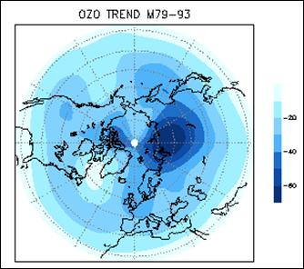
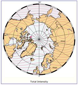
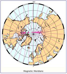
The following figure (left) shows the column ozone trend for March from 1979-1993 [http://jisao.washington.edu/wallace/ncar_notes/]. The adjacent figures show the magnetic field intensity (center) and the magnetic meridians (right) [http://gsc.nrcan.gc.ca/geomag/field/arctics_e.php]. The magnetic field is asymmetrical – with two field maxima: one over the northwest shore of Hudson Bay in Canada, and one over the Central Siberian Plateau. The North Magnetic Pole (NMP) position is indicated by the star. The convergences of the magnetic meridians indicate the approximate path followed by the moving NMP (see http://www.appinsys.com/GlobalWarming/EarthMagneticField.htm). The area of ozone depletion is along the converged magnetic meridians between the two areas of maximum magnetic field intensity.
A 2008 paper by Vogel et al (“Model simulations of stratospheric ozone loss caused by enhanced mesospheric NOx during ArcticWinter 2003/2004”, Atmosheric Chemistry and Physics, 8, 2008 [http://www.atmos-chem-phys.org/8/5279/2008/acp-8-5279-2008.pdf] states: “During periods of solar disturbances solar events can affect the concentration of constituents in the middle atmosphere. Protons, electrons, and alpha particles released from the sun are channelled along the Earth’s magnetic field and cause ionization, excitation, dissociation, and dissociative ionization of the background constituents when they reach the Earth’s atmosphere. Solar disturbances can also lead to solar proton events (SPEs), which are characterized by the emission of protons with higher energies. Some of these highly energetic protons can penetrate to the stratosphere, but generally only in the polar regions.”
|
|
Arctic / Antarctic Ozone Depletion Comparison
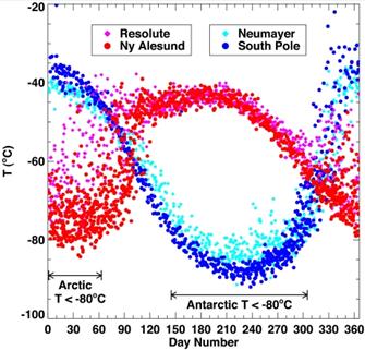
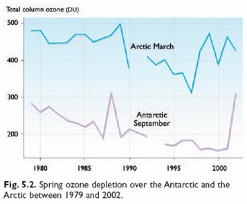
The following figure (left) compares temperatures at 70 (±2) mbar (≈18 km) during ozonesonde ascents in the 1990s for Resolute and Ny Alesund in the Arctic as compared with Neumayer and South Pole in the Antarctic. The portions of the year when temperatures fell below −80°C (the conditions for which ozone depletion chemistry is expected to be most rapid) are also shown [http://www.pubmedcentral.nih.gov/articlerender.fcgi?artid=1761864]. The right-hand figure compares ozone levels for Arctic March and Antarctic September for 1979 – 2002 [http://www.acia.uaf.edu:16080/PDFs/ACIA_Science_Chapters_Final/ACIA_Ch05_Final.pdf].
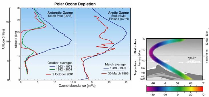
The following figure compares Antarctic and Arctic ozone depletion by altitude (left) [http://www.rsmas.miami.edu/divs/mac/faculty/jrodriquez/seminar_1_29_04.pdf] and a general indication of the variation of temperature with altitude (right).
|
|
Ozone Atmospheric Transport
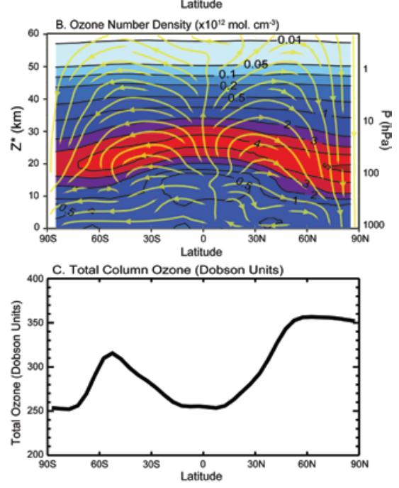
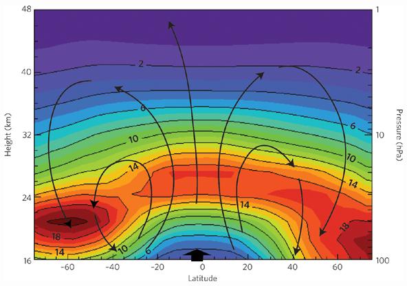
The following figure shows the ozone density by latitude and altitude (top). The yellow lines indicate the atmospheric transport from the equator to the poles (Brewer-Dobson circulation). [http://downloads.climatescience.gov/sap/sap2-4/sap2-4-final-ch3.pdf]
Another schematic of the Brewer-Dobson circulation and the annual mean distributions of ozone. [http://www.nature.com/ngeo/journal/v2/n10/fig_tab/ngeo634_F1.html]
|
|
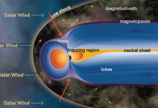
The ozone depletion occurs at the poles because this is where the Earth’s “magnetic field opens up to space, such that solar protons which are energetic enough can get direct access. The trapped electrons in the Van Allen belts are also dumped in the Antarctic atmosphere.” [http://physics.oulu.fi/toiminta/kollokviot/2008-04-10_rodger.pdf] The following figures are from the same reference.
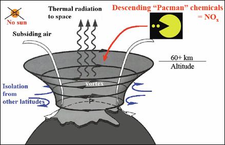
The following figure (also from the above reference) illustrates the effect of the polar vortex. When the sun is absent during the polar winter, the vortex results in charged particles descending into the upper atmosphere and creating NOx molecules which destroy the ozone.
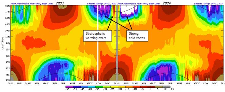
The following figure (also from the above reference) shows the temperature at approximately 50 km altitude for 2003 and 2004.
Figures similar to the above for any year since 1979 are available at [http://www.cpc.ncep.noaa.gov/products/stratosphere/polar/polar.shtml].
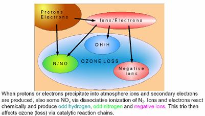
A Finnish paper (“The Long-term Effects of the Oct/Nov 2003 SPEs on Ozone in the Polar Winter Atmosphere” [http://www.cosis.net/abstracts/EGU05/07446/EGU05-A-07446.pdf]) describes the process: “A large solar disturbance like a flare or a coronal mass ejection can result in emission of high-energy protons and other ions from the Sun. If these particles reach the Earth they set off a Solar Proton Event (SPE) during which the charged particles precipitate into the Earth’s atmosphere causing ionization in the middle atmosphere. The effect of the SPEs is confined to the polar cap regions, where the particles are guided by the magnetic field. Ion chemistry leads to increased production of odd nitrogen (NOx = N + NO + NO2) and odd hydrogen (HOx = H + OH + HO2) which participate in catalytic reaction cycles that decrease the amount of ozone in middle atmosphere. HOx gases have a short chemical lifetime but the NOx gases are mainly destroyed by photodissociation. Hence during winter, when little or no sunlight is available in the polar atmosphere, the effect of the NOx cycles can be long-lasting. We have used the nighttime observations of mesospheric and stratospheric O3 and NO2 made by the stellar occultation instrument GOMOS on board the European Space Agency’s Envisat satellite to monitor the increase of NO2 and depletion of ozone due to the SPEs of October-November 2003. The results show NO2 enhancement of several hundred per cent and tens of per cent ozone depletion in the stratopause region, an effect which lasts several months after the events.” Other similar results are described in papers at [http://envisat.esa.int/workshops/ envisatsymposium/sessions/15b.htm].
Figure from: [http://physics.oulu.fi/toiminta/kollokviot/2008-04-10_rodger.pdf] (1: SPE event, 2: NOx descends, 4: energetic electron precipitation, 3: NOx descends)
Ozone is easily depleted in reaction with nitrogen oxides (NOx) in the atmosphere. NOx is produced as a result of solar events. The resulting “destruction of ozone is held in check by Earth’s magnetic field. On the Earth’s surface, the field varies from being horizontal and of magnitude ~ 30,000 nanoTesla (nT) near the equator to vertical and ~ 60,000 nT near the poles. Charged particles are deflected by the horizontal component of the Earth’s magnetic field. Therefore the magnetic shielding of charged particles is strongest above the equator and weakest above the poles.” [http://personals.galaxyinternet.net/tunga/OzoneHole.pdf]
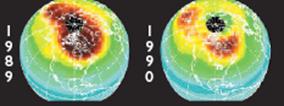
The following figure (left) shows NOx production (top) and ozone depletion (bottom) for an event in 1990 with data for 70 degrees north [http://www.sotere.uni-osnabrueck.de/spacebook/spacebook_files/talks/magneticfieldreversal.pdf]. The adjacent figure to the right shows the ozone depletion as a result (from figure shown previously).
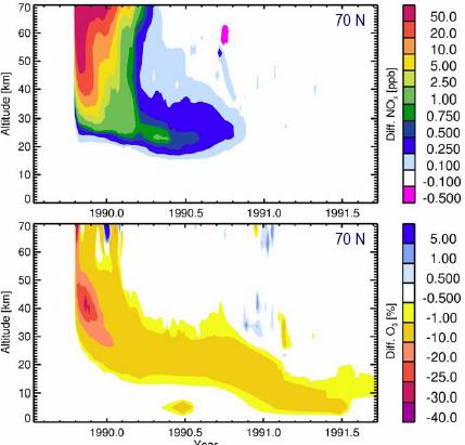
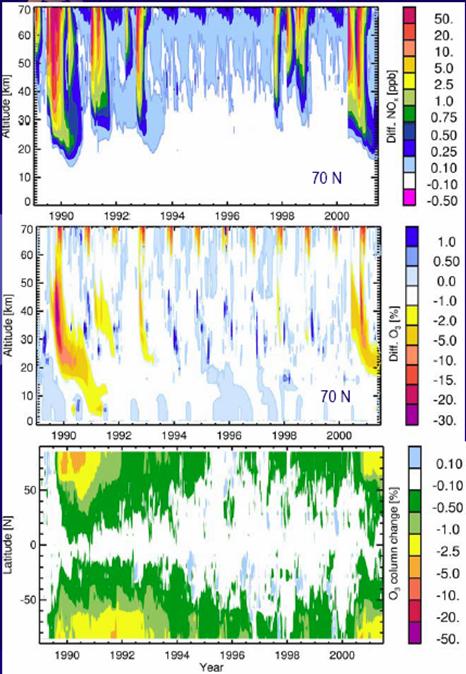
The following figure shows NOx production by altitude (top), ozone depletion by altitude (center) for 70 degrees north and ozone depletion by latitude (bottom) for 1989 to 2001 [http://www.sotere.uni-osnabrueck.de/spacebook/spacebook_files/talks/magneticfieldreversal.pdf]. The NOx events lead the ozone depletion from the upper atmosphere downwards, as shown in the upper and center figures. The events are fairly symmetrical between the poles as indicated in the lower figures.
A 2007 paper (Winkler et al, “Modeling Impacts of Geomagnetic Field Variations on Middle Atmospheric Ozone Responses to Solar Proton Events on Long Timescales”, Journal of Geophysical Research 113 [http://www.agu.org/pubs/crossref/2008/2007JD008574.shtml]) states: “With decreasing magnetic field strength the impacts on the ozone are found to significantly increase especially in the Southern Hemisphere”.
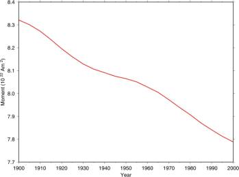
The following figure is from the British Geological Survey [http://www.geomag.bgs.ac.uk/reversals.html], “Measurements have been made of the Earth's magnetic field more or less continuously since about 1840. If we look at the trend in the strength of the magnetic field over this time (for example the so-called 'dipole moment' shown in the graph below) we can see a downward trend. ... We also know from studies of the magnetisation of minerals in ancient clay pots that the Earth's magnetic field was approximately twice as strong in Roman times as it is now.”
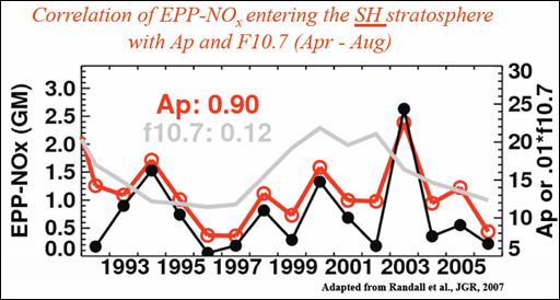
The following figure shows a strong correlation between NOx entering the stratosphere and the geomagnetic index Ap. [http://www.atmosp.physics.utoronto.ca/SPARC/SPARC2008GA/Oral/day3_Hood.pdf]
“Most of the energy transfer to the Earth from the solar wind is accomplished electrically, and nearly the entire voltage associated with this process appears in the polar cap region, which extends typically less than 20° in latitude from the magnetic pole. The total voltage across the polar cap can be as large as 100,000 volts, rivaling that of thunderstorm electrification of the planet in magnitude. This polar cap electric field is the major source of largescale horizontal voltage differences in the atmosphere. Moreover, the dynamic polar region accounts for a large fraction of the variability inherent in our upper atmosphere, variability due to chaotic changes in the solar wind magnetic field that produces large-scale restructuring of the cavity enclosing the Earth’s magnetic field. This restructuring visibly manifests itself most clearly in the production of ionized plasmas and the associated distribution of aurora high over the north and south polar regions. In turn, the Earth’s lower atmosphere (that part responsible for weather phenomena) undergoes variations in composition and dynamics influenced by these coupling effects through a complex and as yet not fully understood feedback system. [http://www.arcus.org/logistics/svalbard/Svalbard.pdf]
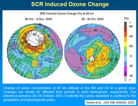
The following figure shows the effects of solar cosmic ray induced ozone depletion in October 2003 [http://ecrs2008.saske.sk/presentations/11-SEP/Fluckiger/2008-ECRS-08-KOSICE-3.ppt]
Much of this has been under investigation for the last couple of decades. A 1992 paper (Bui et al, “Short-period variation of cosmic-ray intensity and ozone density observed in the stratosphere” [http://www.springerlink.com/content/891061284xmx3623/]) states: “The energy deposition by slowing-down of energetic ionizing particles in the atmosphere enhances the production of constituent concentration which perturbs and eventually destroys the ozone (OZ) layer. Near the Brazilian anomaly region the cosmic-ray (CR) intensity varies greatly due to the magnetic activity in that region. In order to study these variations, stratospheric balloons were launched to measure, simultaneously, the CR and OZ fluxes in the atmosphere. The Fourier-analysed data collected during the flight on April 22, 1989 show evidences of a short-period variation for both fluxes measured.”
In 2009, University of Waterloo Professor of Physics and Astronomy, Qing-Bin Lu said [http://newsrelease.uwaterloo.ca/news.php?id=5051] “it was generally accepted for more than two decades that the Earth's ozone layer is depleted by chlorine atoms produced by the sun's ultraviolet light-induced destruction of chlorofluorocarbons (CFCs) in the atmosphere. But mounting evidence supports a new theory that says cosmic rays, rather than the sun's UV light, play the dominant role in breaking down ozone-depleting molecules and then ozone. … Cosmic rays are concentrated over the North and South Poles due to Earth's magnetic field, and have the highest electron-production rate at the height of 15 to 18 km above the ground -- where the ozone layer has been most depleted.”
A 2007 study reported in Nature [http://www.nature.com/news/2007/070924/full/449382a.html] “As the world marks 20 years since the introduction of the Montreal Protocol to protect the ozone layer, Nature has learned of experimental data that threaten to shatter established theories of ozone chemistry. If the data are right, scientists will have to rethink their understanding of how ozone holes are formed and how that relates to climate change. … The rapid photolysis of Cl2O2 is a key reaction in the chemical model of ozone destruction developed 20 years ago. If the rate is substantially lower than previously thought, then it would not be possible to create enough aggressive chlorine radicals to explain the observed ozone losses at high latitudes, says Rex. The extent of the discrepancy became apparent only when he incorporated the new photolysis rate into a chemical model of ozone depletion. The result was a shock: at least 60% of ozone destruction at the poles seems to be due to an unknown mechanism, Rex told a meeting of stratosphere researchers in Bremen, Germany, last week.”
|
|
[Ref. 1] - WMO/UNEP: “SCIENTIFIC ASSESSMENT OF OZONE DEPLETION: 2006” by the SCIENTIFIC ASSESSMENT PANEL OF THE MONTREAL PROTOCOL ON SUBSTANCES THAT DEPLETE THE OZONE LAYER [http://www.wmo.ch/pages/prog/arep/gaw/reports/ozone_2006/pdf/exec_sum_18aug.pdf]
Significant statements from the above report:
|
|
|