Global Warming Science - www.appinsys.com/GlobalWarming
The Greenhouse
[last update: 2011/01/10]
See also: CO2 / IPCC and GHG Emissions - Sources (as well as GHG / Water Vapor)
|
This document contains the following sections:
|
||
|
The Earth’s climate system is very complex and many attempts have been made to model it. There is an interaction of solar radiation and magnetic fields, land, ocean, atmosphere, clouds, gases released by anthropogenic processes (deforestation, agriculture, land use change, burning of carbon-based fuels) and natural processes (volcanoes, etc.). In this system, the sun provides the heating of the earth through solar radiation in various wavelengths. Some of the solar radiation is reflected by clouds, thus reducing the heating from solar radiation (analogy: cloudy days in summer are typically cooler than sunny days because the clouds block heat from the sun). Heat is re-radiated by the Earth’s surface. Some of this heat is absorbed by “greenhouse gases” and re-emitted in the atmosphere, thus contributing to warming the Earth (analogy: cloudy days in winter are typically warmer than sunny days because the clouds keep heat in).
The Sun’s incoming radiation is within the range of visible and near-infrared wavelengths. The Earth’s outgoing radiation is in the longer wavelength spectrum of medium and far-infrared.
The greenhouse effect operates by inhibiting the cooling through reducing the outgoing infrared radiation. The shorter wavelength radiation passes relatively unhindered by greenhouse gases to warm the Earth. The Earth re-radiates the energy in longer wave radiation (infrared, far-infrared) which is absorbed and reradiated by the greenhouse gases, causing atmospheric warming. The following figure provides a simplified conceptual overview of the process.
From: UNEP/GRID-Arendal. Greenhouse effect. UNEP/GRID-Arendal Maps and Graphics Library. 2002. http://maps.grida.no/go/graphic/greenhouse_effect.
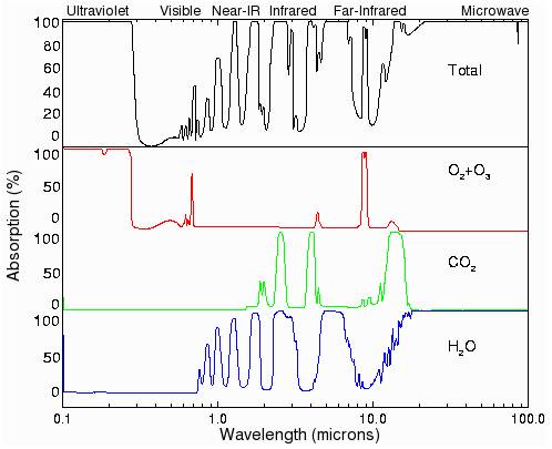
The following figure shows the absorption of radiation by wavelength for H2O, CO2 as well as oxygen and ozone (O2+O3). See http://brneurosci.org/co2.html for a good explanation of the potential global warming effects of CO2.
The following figure shows similar information to the above figure but includes methane and nitrous oxide, as well as showing the effect on the incoming and outgoing radiation (Wikipedia).
One of the major points of the above is that water vapor is by far the main greenhouse gas keeping the atmosphere warm. This reduces the role that additional greenhouse gases can play since they are not independent.
The most important greenhouse gases in Earth's atmosphere include water vapor (H2O), carbon dioxide (CO2), methane (CH4), nitrous oxide (N2O), ozone (O3), and the chlorofluorocarbons (CFCs). In addition to reflecting sunlight, clouds are also a major greenhouse substance. Water vapor and cloud droplets are in fact the dominant atmospheric absorbers. Water vapor is the most important greenhouse gas due to its abundance in the atmosphere.
The relationship between CO2 and increased temperature has been demonstrated in laboratory experiments and shown to be a logarithmic relationship – i.e. one must keep doubling the concentration to achieve the same increment of warming. The effect of doubling the CO2 has been estimated to be approximately 0.7 C. However that does not take into account the presence of other greenhouse gases (GHG). Water vapor is the most prevalent GHG and the effect of increasing CO2 depends on the relative quantity of non-CO2 GHG. Thus in humid atmospheric conditions, CO2 contributes very little warming, whereas it could contribute more in dry atmospheric regions.
As a result of the logarithmic effect of increase in GHG, doubling the atmospheric CO2 from 300 to 600 ppm has virtually no effect on preventing outgoing radiation because it is a very small component compared to water vapor, as shown in the following figure [http://en.wikipedia.org/wiki/Radiative_forcing]
The only way that climate models can achieve significant warming from increasing CO2 is through a theoretical positive feedback mechanism that increases water vapor.
Richard Lindzen (MIT Atmospheric Science Professor) states: “there is a much more fundamental and unambiguous check of the role of feedbacks in enhancing greenhouse warming that also shows that all models are greatly exaggerating climate sensitivity. Here, it must be noted that the greenhouse effect operates by inhibiting the cooling of the climate by reducing net outgoing radiation. However, the contribution of increasing CO2 alone does not, in fact, lead to much warming (approximately 1 deg. C for each doubling of CO2). The larger predictions from climate models are due to the fact that, within these models, the more important greenhouse substances, water vapor and clouds, act to greatly amplify whatever CO2 does. This is referred to as a positive feedback. It means that increases in surface temperature are accompanied by reductions in the net outgoing radiation – thus enhancing the greenhouse warming. ... Satellite observations of the earth’s radiation budget allow us to determine whether such a reduction does, in fact, accompany increases in surface temperature in nature. As it turns out, the satellite data from the ERBE instrument (Barkstrom, 1984, Wong et al, 2006) shows that the feedback in nature is strongly negative -- strongly reducing the direct effect of CO2 (Lindzen and Choi, 2009) in profound contrast to the model behavior.” [http://www.quadrant.org.au/blogs/doomed-planet/2009/07/resisting-climate-hysteria]
|
||
|
NOAA had a “Weather School” “Learning Lesson” web page with a CO2 experiment (it has since been removed but can still be viewed at: [http://web.archive.org/web/20060129154229/http://www.srh.noaa.gov/srh/jetstream/atmos/ll_gas.htm]). The web page is shown below (originally at: [http://www.srh.noaa.gov/srh/jetstream/atmos/ll_gas.htm] – removed in Nov. 2009) [Red highlighting added.]
|
||
|
The temperature varies with altitude. The following
figure provides a general indication of the variation of temperature with
altitude and indicates the parts of the atmosphere referred to as the
troposphere and the stratosphere. The stratosphere is warmer due to
increased ozone levels absorbing ultraviolet radiation. The greenhouse
gas (GHG) theory indicates that increasing GHGs should result in warming
of the troposphere and cooling of the stratosphere. Temperature Variation By Altitude
|
||
|
Carbon Cycle
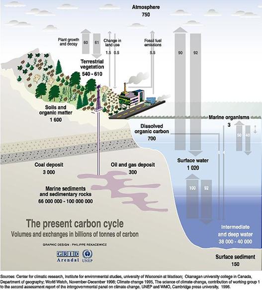
The global carbon cycle involves reservoirs of carbon deposits along with exchanges of carbon between sources / sinks and the atmosphere on an annual fluctuation. The following figure shows the generalized global carbon cycle from UNEP (IPCC 1996) [http://www.grida.no/publications/vg/climate/page/3066.aspx] It shows “carbon reservoirs in GtC (gigatonne= one thousand million tonnes) and fluxes in GtC/year. The indicated figures are annual averages over the period 1980 to 1989.”
The fossil fuel emissions total is dwarfed by the annual exchanges between the terrestrial and oceanic cycles. The fossil fuel emissions total is the easiest number to calculate in this figure. The rest are subject to gross estimates not indicated in the figure. The figure caption in the source states: “Evidence is accumulating that many of the fluxes can fluctuate significantly from year to year. In contrast to the static view conveyed in figures like this one, the carbon system is dynamic and coupled to the climate system on seasonal, interannual and decadal timescales.” In other words, attribution of atmospheric CO2 increase to fossil fuels over the last 50 years, since consistent measurements began, is not supported by the lack of knowledge in actual cycle fluctuations.
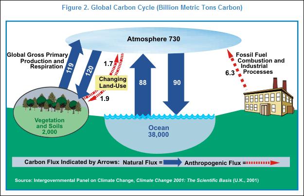
The following figure shows the carbon cycle from the IPCC 2001 as displayed on the US government’s Energy Information Administration web site [http://www.eia.doe.gov/oiaf/1605/ggccebro/chapter1.html]. “Given the natural variability of the Earth’s climate, it is difficult to determine the extent of change that humans cause. … there is uncertainty in how the climate system varies naturally and reacts to emissions of greenhouse gases. we cannot rule out that some significant part of these changes is also a reflection of natural variability.”
Note that they do not include the level of uncertainty in the estimates in the above figures.
|
||
|
Many scientists disagree that past atmospheric CO2 has been historically constantly low, as the IPCC states. The IPCC rejected all available historical measurements of CO2, except Antarctic ice cores, because the measurements did not match their preferred theory. An examination of the history of CO2 measurement is provided at http://www.co2web.info/ESEF3VO2.pdf
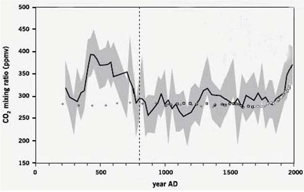
Reconstructions of past CO2 (prior to continuous measurements) have been made from various sources. The IPCC uses reconstruction from ice cores. Other reconstructions show different trends. The following figure shows CO2 reconstruction from pine needle stomatal density. [http://icecap.us/images/uploads/200705-03AusIMMcorrected.pdf]
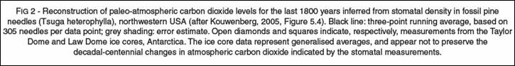
Although the IPCC rejected all available historical measurements of CO2, except Antarctic ice cores, “more than 90,000 direct measurements of CO2 in the atmosphere, carried out in America, Asia, and Europe between 1812 and 1961, with excellent chemical methods (accuracy better than 3%), were arbitrarily rejected”. Even the ice core measurements were adjusted to match their CO2 story line, as shown in the following figure. [http://www.warwickhughes.com/icecore/zjmar07.pdf]
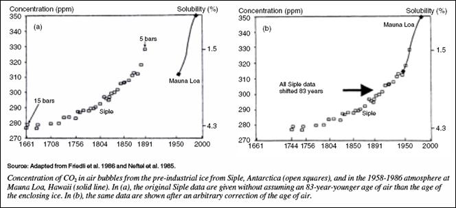
A CO2 reconstruction study based on oak tree leaf stomata in the Netherlands (van Hoof et al “A Role for Atmospheric CO2 in Preindustrial Climate Forcing”, Proceedings of the US National Academy of Sciences, 2007) shows the following figure comparing the study findings (red line) with the IPCC findings (blue line) in terms of the CO2 climate forcing. [http://www.pnas.org/content/105/41/15815.full.pdf+html] The study states: “Comparable to other stomata-based records, reconstructed preindustrial CO2 levels fluctuate between 319.2 and 292.3 ppmv with an average value of 311.4 ppmv … It should be noted that, in general, CO2 data derived from stomatal frequency analysis have higher average values (300 ppmv) compared with the IPCC baseline ”
For further information on historical CO2 measurements, see:
|
||
|
The atmospheric CO2 has been shown to lag the temperature in the past ice-age / warming cycles, as shown in the following figure (From http://calspace.ucsd.edu/virtualmuseum/climatechange2/07_2.shtml). What is not visually evident frm the graph is that CO2 increase follows the temperature, as discussed below.
Vostok Ice Core Temperature and CO2 Trends for Past 450,000 Years
The IPCC AR4 Scientific Basis report, Part 6 (May 2007), makes the following statements:
Many scientific studies have shown that CO2 increase follows temperature increase in the pre-historical records. A few examples:
|
||
|
The NOAA Earth System Research Laboratory – Global Monitoring Division [http://www.esrl.noaa.gov/gmd/aggi/] provides data from a network of CO2 monitoring stations around the world (with data for Mauna Loa starting in 1970). The following figures show the location of the monitoring locations (left) and the global average CO2 concentration from these sites (right).
NOAA/ESRL CO2 Monitoring Locations (Left) and Global Average CO2 Concentration (Right)
The following figure shows the IPCC graph of atmospheric CO2 as measured at Mauna Loa, Hawaii (left), while the right-hand graph compares the CO2 at Mauna Loa and the South Pole. They show a similar trend in slope. In fact the CO2 plots from any of the CO2 stations in the NOAA database show a similar CO2 trend. It can be seen from the figure below that the CO2 is greater in the summer than the winter (the CO2 is not causing seasons, but it is a response to the seasonal change in temperature).
Comparing the various CO2 trends available from the NOAA database shows a consistent trend in atmospheric CO2 rise around the world (as illustrated by comparing the figures shown above and below). But the temperature trends vary greatly by region.
Left: Atmospheric CO2 at Mauna Loa (Figure 2.3 in the IPCC AR4) Right: Atmospheric CO2 at Mauna Loa (Red) and at South Pole (Blue) from the NOAA Database
The temperature trend at Mauna Loa shows no correspondence with the CO2 trend. The following figure shows the Mauna Loa CO2 along with the temperature trend from the nearest station in the NASA GISS database (Hilo, Hawaii) clearly illustrating the lack of correspondence between the two.
Atmospheric CO2 at Mauna Loa (Figure 2.3 in the IPCC AR4) with Temperature Trend from the NASA GISS Database for Hilo.
|
||
|
CO2 – Ocean Water Relationship
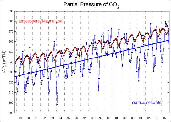
The following figure compares the atmospheric CO2 and ocean surface CO2 at a station in Hawaii. [http://hahana.soest.hawaii.edu/hot/trends/trends.html] It shows the inverse annual correlation between atmospheric and sea surface CO2 – within each year the cycle is opposite.
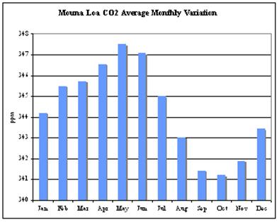
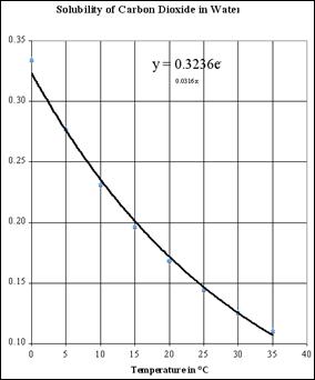
The following figure shows the monthly variation in CO2 at Mauna Loa (left) and the solubility of CO2 in water as a function of temperature [from http://wattsupwiththat.com/2007/11/04/guest-weblog-co2-variation-by-jim-goodridge-former-california-state-climatologist/]. Seasonal changes in CO2 are a result of seasonal CO2 sources and sinks in the global carbon cycle. The ocean temperature plays a large role in this, as shown previously in the Carbon Cycle section.
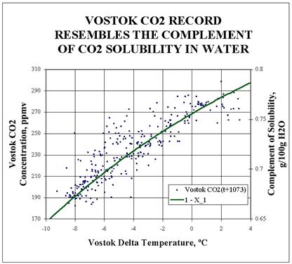
An analysis of the Vostok CO2 data [http://www.rocketscientistsjournal.com/2006/10/co2_acquittal.html] provides the following figure comparing the Vostok CO2 versus temperature change with the complement of CO2 solubility in water (i.e. 1 minus the solubility shown above)
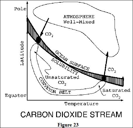
Based on the solubility relationship displayed in the Vostok data, the following model is suggested at [http://www.rocketscientistsjournal.com/2006/10/co2_acquittal.html]: “The shaded area represents the interface of the ocean surface layer with the atmosphere. The ocean has circulation components that carry light weight water poleward in the surface layer, cooling along the way and thus absorbing more CO2 as Henry's Law requires. It becomes more dense as it cools and is freshened from land runoff in the classical model. But as shown here, it also increases in density as it loads with CO2. It's the surface component of a ThermoHaline Carbon Circulation, THCC. The subsurface component is labeled as the Conveyor Belt. The THCC headwaters are at the poles, where it has a CO2 concentration corresponding to a perpetual temperature of 0ºC to 4ºC, and proportional to the existing CO2 concentration in the atmosphere. The THCC emerges at the surface approximately one millennium later to outgas according to Henry's Law in proportion to the CO2 concentration and surface temperature at the time and place of discharge. The bulk of this outgassing, perhaps 80%, occurs in the Eastern Equatorial Pacific. Thus the hypothesis is that the volume of CO2 outgassed by the ocean is proportional to the CO2 content then, a millennium ago, and the sea surface temperature now.”
|
||
|
CO2 – Temperature Observations
The following figure compares satellite-based lower troposphere temperature (blue) with CO2 growth rate (black) for 1979 - 2008. The temperature changes precede the CO2 growth rate changes.
The following figure shows a regression of CO2 growth as a function of temperature calculated from points in the above figure [from http://icecap.us/images/uploads/FlaticecoreCO2.pdf].
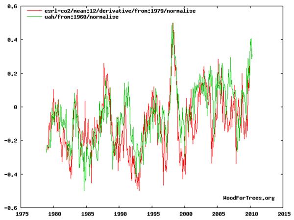
A similar graph to the time series plot two graphs above can be produced with current data at [http://www.woodfortrees.org/plot/esrl-co2/mean:12/derivative/from:1979/normalise/plot/uah/from:1960/normalise] as shown below
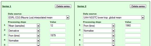
Interactive graph settings for the above at WoodForTrees:
|
||
|
The positive effects of increased atmospheric CO2 are ignored in the alarmist scare stories.
The UN periodically produces an assessment of the worldwide ozone depletion. The most recent report: WMO/UNEP: “Scientific Assessment of Ozone Depletion: 2006” by the Scientific Assessment Panel of the Montreal Protocol on Substances that Deplete the Ozone Layer [http://www.wmo.ch/pages/prog/arep/gaw/reports/ozone_2006/pdf/exec_sum_18aug.pdf] states: “Model simulations suggest that changes in climate, specifically the cooling of the stratosphere associated with increases in the abundance of carbon dioxide, may hasten the return of global [(60°S-60°N)] column ozone to pre-1980 values by up to 15 years”. Perhaps CO2 isn’t all-bad.
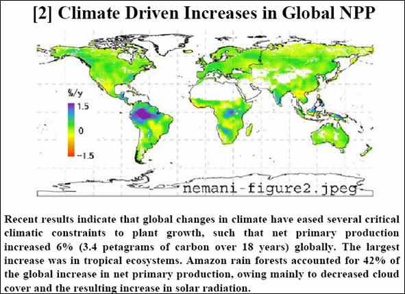
Vegetation – Net Primary Productivity
The following figure is from the United Nations UNEP [http://maps.grida.no/go/graphic/losses-in-land-productivity-due-to-land-degradation] showing a substantial increase in global productivity from 1981 – 2003 (interestingly, the UNEP’s caption was “losses in land productivity due to land degradation” – typical of the UN’s cup-half-empty viewpoint).
The following figure is from a study “Long Term Monitoring of Vegetation Greenness from Satellites” [http://www.ias.sdsmt.edu/STAFF/INDOFLUX/Presentations/14.07.06/session1/myneni-talk.pdf]
A study of tree growth in Maryland indicates that “forests in the Eastern United States are growing faster than they have in the past 225 years” and is attributed to increased CO2 [http://sercblog.si.edu/?p=466]
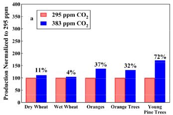
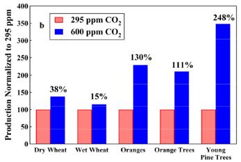
Agriculture
Studies of crop growth rates under various concentrations of CO2 also show a positive effect of the current increase in atmospheric CO2. The following figures show an example.
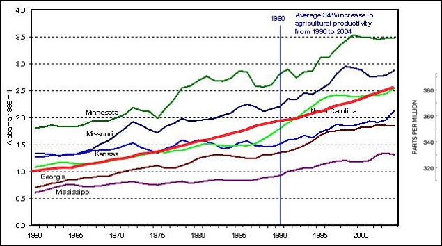
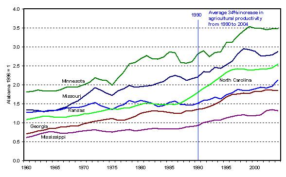
The USDA provides agricultural productivity data [http://www.ers.usda.gov/Data/AgProductivity/table03.xls] listing state-by-state yearly data. The data has been graphed by David Archibald [http://icecap.us/images/uploads/STATESPRODUCTIVITY.JPG] and is shown below for 1960 to 2005 for several states. I have added the thick red line showing atmospheric CO2 at Mauna Loa over the same time period (CO2 graph from http://www.esrl.noaa.gov/gmd/ccgg/trends/co2_data_mlo.html).
Agricultural Productivity for Six States, Plus Atmospheric CO2 (Red – Scale at right)
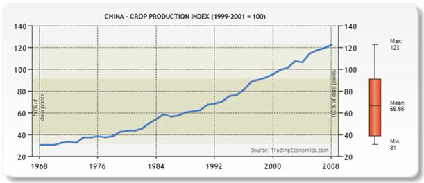
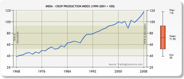
The following figures show crop production in China and India for 1968-2009 (“Crop production index shows agricultural production for each year relative to the base period 1999-2001. It includes all crops except fodder crops.” [http://tradingeconomics.com/china/crop-production-index-1999-2001--100-wb-data.html])
Studies of peanut growth in the United States have found increased crops with elevated CO2. For example a study of the effects of increase O3 (ozone) and CO2 [http://crop.scijournals.org/cgi/content/abstract/47/4/1488] found: “adverse effects of tropospheric O3 on C3 crop plants are ameliorated by elevated concentrations of atmospheric CO2”
Another 2009 study [http://www.plantphysiol.org/cgi/reprint/151/3/1009] states: “Growth at elevated [CO2] stimulates photosynthesis and increases carbon (C) supply in all C3 species.”
Agricultural productivity has been increasing in most of Africa. Africa’s problems are not due to US CO2 emissions causing “climate change”. According to a UN report: “Africa has 733 million hectares of arable land (27.4 per cent of world total) compared with 570 million hectares for Latin America and 628 million hectares for Asia. Only 3.8 per cent of Africa’s surface and groundwater is harnessed, while irrigation covers only 7 per cent of cropland (3.6 per cent in SSA). Clearly, there is considerable scope for both horizontal and vertical expansion in African agriculture. … Insecurity in land ownership has been blamed for accelerated land degradation and lack of long-term investments in sustainable land management and stewardship of natural resources.” Like most studies of Africa agricultural problems, the UN report recommends “Increase fertilizer use from the low levels of 125 gm/ha to at least 500 gm/ha, which is about half of the world average, and increasingly aim to reach the world average. …Strategies for transforming African agriculture have to address such challenges as low investment and productivity, poor infrastructure, lack of funding for agricultural research, inadequate use of yield-enhancing technologies” [http://www.uneca.org/era2009/chap4.pdf]
See: IPCC Misleads on African Agriculture: http://www.appinsys.com/GlobalWarming/IPCC_AfricaCrops.htm
See also: Increasing Arctic Plant Biomass: http://www.appinsys.com/globalwarming/GW_4CE_Animals.htm#arcticplant
|
||
|
|


